Lisheng Xie - Blog - 算法学习 2024-01-29T21:56:45+08:00 Typecho https://www.lishengxie.top/index.php/feed/atom/category/%25e7%25ae%2597%25e6%25b3%2595%25e5%25ad%25a6%25e4%25b9%25a0/ <![CDATA[Leetcode刷题 - KMP算法]]> https://www.lishengxie.top/index.php/archives/194/ 2024-01-29T21:56:45+08:00 2024-01-29T21:56:45+08:00 lishengxie https://www.lishengxie.top/ KMP算法是一种高效的字符串匹配算法,但是之前每次学过之后都会忘记,这次做一下总结加深印象,主要参考了以下链接。

问题

给定一个字符串$s$(长度为N)和一个模式串$t$(长度为M),如果$s$中存在$t$,那么返回模式串第一次出现的起始索引;如果不存在返回-1。对应Leetcode 28. 找出字符串中第一个匹配项的下标

KMP算法

KMP算法是由D.E.Knuth,J.H.Morris和V.R.Pratt同时发现的一种快速的字符串匹配算法,时间复杂度为$O(M+N)$。KMP算法的核心思想是在字符串匹配失败时利用之前已经匹配的信息来做快速回退,避免从头再做匹配。KMP算法的核心函数是一个用于求解next数组的函数,next数组包含了模式串局部匹配的信息。

这里代码随想录中给出了关于next数组的详细解释。next数组对应自定义的前缀表,其中前缀表是一个和模式串长度相同的数组,前缀表第i个位置的值为[0,i]子字符串的最长相同前后缀的长度;

  • 前缀是指不包含最后一个字符的所有以第一个字符开头的连续子串。后缀是指不包含第一个字符的所有以最后一个字符结尾的连续子串;
  • 举例来说,“aab”的前缀有“a”和“aa”、后缀有“b”和“ab”,“aabaa”的最长相同前后缀长度为2,“aa”的最长相同前后缀长度为1。

以下图为例,假设文本串和模式串分别为aabaabaafaaabaaf,前缀表如图中所示。那么在bf不匹配时,此时寻找前缀表中前一位存储的值,查找得到值为2,该值的含义是“aabaa”的最长相同前后缀长度为2,即“aa”。此时我们可以不用从头开始重新匹配,文本串中的匹配指针可以不移动,将模式串中的匹配指针回退到索引2处重新开始匹配即可。
prefix table

  • 这里为什么可以不回退文本串的匹配指针?

    因为这里通过回退j指针,找到了从文本串中该位置向前的最长相同前后缀,获得了类似下图的效果。

prefix table

  • 实际使用中常通过将前缀表统一减1得到next数组,那么如何计算next数组?

    next数组的计算类似于移动模式串,在模式串和模式串之间做匹配,在移动的过程中计算next数组的值,next数组的计算代码如下所示:
    void getNext(int* next, const string& s){
      int j = -1;
      next[0] = j;
      for(int i = 1; i < s.size(); i++) { // 注意i从1开始
          while (j >= 0 && s[i] != s[j + 1]) { // 前后缀不相同了
              j = next[j]; // 向前回退
          }
          if (s[i] == s[j + 1]) { // 找到相同的前后缀
              j++;
          }
          next[i] = j; // 将j(前缀的长度)赋给next[i]
      }
    }
  • 基于next数组进行文本串和模式串的匹配代码如下:

    void match(string s, string t) {
      int j = -1;
      int next[t.size()];
      getNext(next, t);
    
      for (int i = 0; i < s.size(); i++) {
          while (j >= 0 && s[i] != t[j+1]) {
              j = next[j];
          }
          if (s[i] == s[j+1]) {
              j++;
          }
          if (j == (t.size() - 1)) {
            return i - t.size() + 1;
          }
      }
      return -1;
    }
]]>
<![CDATA[算法学习 - 差分数组]]> https://www.lishengxie.top/index.php/archives/178/ 2023-12-21T14:52:00+08:00 2023-12-21T14:52:00+08:00 lishengxie https://www.lishengxie.top/

差分数组

问题描述

给定一个数组,需要频繁地对某个区间内的元素做加减操作,并获取最后的操作结果。常规做法是每次都遍历整个区间然后修改区间内的元素,但是元素的访问需要时间、频繁访问元素会减慢程序的运行时间。因此,可以使用差分数组来进行优化。

一维差分数组定义

一维差分数组$ d[n] $定义为原始数组$ nums $相邻元素之间的差,即$d[i]=nums[i]-nums[i-1]$,其中$d[0]=nums[0]$。这样原数组就是差分数组的前缀和

$$ nums[i] = \sum_{k=0}^i d[k]. $$

由此,我们可以改进原来的区间操作,如对区间$[a,b]$内每个元素加3,那么只需要在区间的两端进行操作即可,即

$$ d[a] += 3, d[b+1] -= 3 $$

证明

假设$nums1$是修改后的数组,$d1$是修改后的差分数组,其中$d1[a]=d[a]+3, d1[b+1]=d[b+1]-3$.

  • 对于$0\leq i \lt a$, $nums1[i] = \sum_{k=0}^i d1[k] = \sum_{k=0}^i d[k] = nums[i]$.
  • 对于$a\leq i \leq b$,

    $$ \begin{align} nums1[i] &= \sum_{k=0}^i d1[k] \\&= \sum_{k=0}^{a-1}d[k] + \sum_{k=a+1}^{b}d[k] + d[a] + 3 \\&= \sum_{k=0}^i d[k] + 3 \\&= nums[i]+3 \end{align}. $$

  • 对于$i \gt b$,

    $$ \begin{align} nums1[i] &= \sum_{k=0}^i d1[k]\\ &= \sum_{k=0}^{a-1}d[k] + \sum_{k=a+1}^{b}d[k] + \sum_{k=b+1}^{i}d[k] + d[a] + 3 + d[b] - 3\\ &= \sum_{k=0}^i d[k] + 3 - 3\\ &= nums[i]. \end{align} $$

    由此,可以证明只修改差分数组的两端即可以修改原数组的整个区间。

代码

class Solution {
public:
    vector<int> diff;
    vector<int> nums;

    void diffNums() {
        diff[0] = nums[0];
        for(int i = 1; i < nums.size(); ++i) {
            diff[i] = nums[i] - nums[i-1];
        }
    }

    void increment(int a, int b, int val) {
        diff[a] += val;
        if (b + 1 < diff.size())
            diff[b + 1] -= val;
    }

    void result() {
        nums[0] = diff[0];
        for (int i = 1; i < diff.size(); i++)
            nums[i] = diff[i] + nums[i - 1];
    }

    vector<int> corpFlightBookings(vector<vector<int>>& bookings, int n) {
        nums.resize(n, 0);
        diff.resize(n, 0);
        diffNums();
        for (int i = 0; i < bookings.size(); ++i) {
            increment(bookings[i][0]-1, bookings[i][1]-1, bookings[i][2]);
        }
        result();
        return nums;
    }
};

拓展 - 二维差分数组

二维差分数组可以在一维差分数组的基础上进行拓展,视为一个平面,定义如下

$$ d[i][j] = nums[i][j] - nums[i-1][j] - nums[i][j-1] + nums[i-1][j-1] $$

那么相应地

$$ nums[i][j] = nums[i-1][j] + nums[i][j-1] - nums[i-1][j-1] + d[i][j] $$

假设以 $(x1,y1)$ 为左上角, $(x2,y2)$ 为右下角构成一个区间$S$,如果对这个区间内的每个元素增加$val$,只需要执行下面四步即可。

$$ \begin{align} &d[x1][y1] += val \\ &d[x1][y2+1] -= val \\ &d[x2+1][y1] -= val \\ &d[x2+1][y2+1] += val \end{align} $$

证明

同样假设$num1$和$d1$是修改后的数组和查分数组,以下分情况进行讨论

  • 对于$(m,n)$满足$m<x1$或$n<y1$, 容易知道该范围内查分数组未发生变化,求解该范围内的数组不需要用到区间$S$内的差分数组,因此该范围内数组不受影响;
  • 对于$(m,n)\in S$, 不妨设原数组$num$的元素均为$a$, 那么

    $$ \begin{align} nums1[x1][y1] &= nums1[x1-1][y1] + nums1[x1][y1-1] - nums1[x1-1][y1-1] + d1[x1][y1]\\ &= nums[x1-1][y1] + nums[x1][y1-1] - nums[x1-1][y1-1] + d[x1][y1] + val\\ &= nums[x1][y1] + val; \end{align} $$

    对于$S$内的其他点,使用此递推公式同样可以推导出

    $$ nums1[m,n] = nums[m][n]+val $$

  • 对于$(m,n)$满足$x1\leq m \leq x2$且$n\gt y2$, 我们可以知道

    $$ \begin{align} nums1[x1][y2+1] &= nums1[x1-1][y2+1] + nums1[x1][y2] - nums1[x1-1][y2] + d1[x1][y2+1]\\ &= nums[x1-1][y2+1] + nums[x1][y2] + val - nums[x1-1][y2] + d[x1][y2+1] - val\\ &= nums[x1][y2+1]; \end{align} $$

    对于其他$(m,n)$使用递推公式同样可以发现数组的值没有发生变化。

  • 对于$(m,n)$满足$m\gt x2$且$y1\leq n \leq y2$, 可以使用类似上一种情况的方式推导发现数组数值未发生变化;
  • 最后,对于$(m,n)$满足$m\gt x2$且$n\gt y2$,我们考虑

    $$ \begin{align} nums1[x2+1][y2+1] &= nums1[x2][y2+1] + nums1[x2+1][y2] - nums1[x2][y2] + d1[x2+1][y2+1]\\ &= nums[x2][y2+1] + nums[x2+1][y2] - nums[x2][y2] - val + d[x2+1][y2+1] + val\\ &= nums[x2+1][y2+1]; \end{align} $$

    对于该区域其他点可以类推。

由此,我们得到,差分数组定义以及更新方式满足条件。

代码(来自参考链接)

// Java代码,需要注意边界情况
private int[][] d;// 差分数组。
private int[][] a;// 原数组。

public TwoDiffNums(int[][] a) {
    this.a = a;
    int m = a.length;
    int n = a[0].length;
    d = new int[m][n];
    // 求差分数组。
    for (int i = 0; i < m; i++)
        for (int j = 0; j < n; j++)
            add(i, j, i, j, a[i][j]);
}

public void add(int x1, int y1, int x2, int y2, int val) {
    d[x1][y1] += val;
    if (y2 + 1 < d[0].length)
        d[x1][y2 + 1] -= val;
    if (x2 + 1 < d.length)
        d[x2 + 1][y1] -= val;
    if (x2 + 1 < d.length && y2 + 1 < d[0].length)
        d[x2 + 1][y2 + 1] += val;
}

// 返回结果数组。
public int[][] result() {
    for (int i = 0; i < a.length; i++) {
        for (int j = 0; j < a[0].length; j++) {
            int x1 = i > 0 ? a[i - 1][j] : 0;
            int x2 = j > 0 ? a[i][j - 1] : 0;
            int x3 = i > 0 && j > 0 ? a[i - 1][j - 1] : 0;
            a[i][j] = x1 + x2 - x3 + d[i][j];
        }
    }
    return a;
}
]]>
<![CDATA[LeetCode刷题-二叉树遍历迭代法]]> https://www.lishengxie.top/index.php/archives/160/ 2023-10-08T16:29:19+08:00 2023-10-08T16:29:19+08:00 lishengxie https://www.lishengxie.top/

LeetCode题目链接

二叉树的前序遍历:https://leetcode.cn/problems/binary-tree-preorder-traversal/
二叉树的中序遍历:https://leetcode.cn/problems/binary-tree-inorder-traversal/
二叉树的后序遍历:https://leetcode.cn/problems/binary-tree-postorder-traversal/

二叉树的遍历方法有两种,分别是递归法和迭代法;实际使用中由于系统调用栈有限制,使用递归法可能会导致栈溢出,这里记录三种遍历的迭代做法。最后,介绍二叉树层序遍历的两种方法。

迭代遍历法借助辅助栈实现,下面是二叉树节点的定义,使用链表实现。

 struct TreeNode {
     int val;
     TreeNode *left;
     TreeNode *right;
     TreeNode() : val(0), left(nullptr), right(nullptr) {}
     TreeNode(int x) : val(x), left(nullptr), right(nullptr) {}
     TreeNode(int x, TreeNode *left, TreeNode *right) : val(x), left(left), right(right) {}
 };

前序遍历

前序遍历的顺序是中左右,每次先处理中间节点,那么先将根节点入栈,然后将右孩子入栈,再将左孩子入栈。先右后左的原因是因为入栈顺序和处理顺序是相反的。前序遍历的处理代码如下:

class Solution {
public:
    vector<int> preorderTraversal(TreeNode* root) {
        vector<int> res;
        stack<TreeNode*> st;
        if (root == NULL) {
            return res;
        }

        st.push(root);
        while (!st.empty()) {
            TreeNode *cur = st.top();
            st.pop();
            res.push_back(cur->val);
            if (cur->right) st.push(cur->right);
            if (cur->left) st.push(cur->left);
        }

        return res;
    }
};

中序遍历

中序遍历处理顺序为左中右,先访问二叉树顶部的节点,随后逐层向下访问直到树最左侧的节点,再开始处理节点,这导致处理节点的顺序和访问节点的顺序不一致。中序遍历的迭代法如下所示:

class Solution {
public:
    vector<int> inorderTraversal(TreeNode* root) {
        vector<int> res;
        stack<TreeNode*> st;
        if (root == NULL) {
            return res;
        }
        TreeNode *cur = root;
        while (cur!=NULL || !st.empty()) {
            if (cur != NULL) {
                if (cur) st.push(cur);
                cur = cur->left;
            } else {
                cur = st.top();
                st.pop();
                res.push_back(cur->val);
                cur = cur->right;
            }
        }
        return res;
    }
};

后序遍历

先序遍历是中左右,后续遍历是左右中,那么只需要调整一下先序遍历的代码顺序,就变成中右左的遍历顺序,然后在反转result数组,输出的结果顺序就是左右中了。后序遍历的代码如下所示:

class Solution {
public:
    vector<int> postorderTraversal(TreeNode* root) {
        vector<int> res;
        stack<TreeNode*> st;
        if (root == NULL) {
            return res;
        }
        st.push(root);
        while (!st.empty()) {
            TreeNode *cur = st.top();
            st.pop();
            if (cur->left) st.push(cur->left);
            if (cur->right) st.push(cur->right);
            res.push_back(cur->val);
        }
        reverse(res.begin(), res.end());
        return res;   
    }
};

统一的迭代遍历法

参考https://programmercarl.com/%E4%BA%8C%E5%8F%89%E6%A0%91%E7%9A%84%E7%BB%9F%E4%B8%80%E8%BF%AD%E4%BB%A3%E6%B3%95.html
每次在待处理节点入栈后,加入一个NULL节点作为标记,之后在遇到NULL节点时处理栈中的下一个节点。需要注意的是,这种方法效率不高,节点可能会多次入栈。

层序遍历

// 迭代遍历,BFS基于队列
class Solution {
public:
    vector<vector<int>> levelOrder(TreeNode* root) {
        vector<vector<int>> res;
        queue<TreeNode*> q;
        if (root == NULL)  {
            return res;
        }

        q.push(root);
        while (!q.empty()) {
            int size =q.size();
            vector<int> layer;
            for (int i = 0; i < size; ++i) {
                TreeNode *cur = q.front();
                q.pop();
                layer.push_back(cur->val);
                if (cur->left) q.push(cur->left);
                if (cur->right) q.push(cur->right);
            }
            res.push_back(layer);
        }
        return res;
    }
};

// 递归,DFS
class Solution {
public:
    vector<vector<int>> levelOrder(TreeNode* root) {
        vector<vector<int>> res;
        queue<TreeNode*> q;
        if (root == NULL)  {
            return res;
        }

        order(0, root, res);
        return res;
    }

    // DFS, 递归
    void order(int depth, TreeNode *cur, vector<vector<int>> &res) {
        if (cur == NULL) return;
        if (res.size() == depth) res.push_back(vector<int>());
        res[depth].push_back(cur->val);
        order(depth + 1, cur->left, res);
        order(depth + 1, cur->right, res);
    }
};
]]>
<![CDATA[LeetCode刷题 - 滑动窗口最大值]]> https://www.lishengxie.top/index.php/archives/158/ 2023-10-06T11:45:00+08:00 2023-10-06T11:45:00+08:00 lishengxie https://www.lishengxie.top/ 参考链接:https://programmercarl.com/0239.%E6%BB%91%E5%8A%A8%E7%AA%97%E5%8F%A3%E6%9C%80%E5%A4%A7%E5%80%BC.html

leetcode题目链接:https://leetcode.cn/problems/sliding-window-maximum/

给你一个整数数组 nums,有一个大小为 k 的滑动窗口从数组的最左侧移动到数组的最右侧。你只可以看到在滑动窗口内的 k 个数字。滑动窗口每次只向右移动一位。

返回滑动窗口中的最大值 。

示例 1:

输入:nums = [1,3,-1,-3,5,3,6,7], k = 3
输出:[3,3,5,5,6,7]
解释:

滑动窗口的位置最大值
[1 3 -1] -3 5 3 6 73
1 [3 -1 -3] 5 3 6 73
1 3 [-1 -3 5] 3 6 75
1 3 -1 [-3 5 3] 6 75
1 3 -1 -3 [5 3 6] 76
1 3 -1 -3 5 [3 6 7]7

示例 2:

输入:nums = [1], k = 1 输出:[1]

方法1:单调队列法

使用一个数据结构,每次滑动窗口时添加一个元素,删除一个元素,同时可以从队列头部获取想要的当前窗口内的最大值。这种数据结构就是单调队列,单调队列的pop和push操作应该遵循以下原则:

  1. pop(value):如果窗口移除的元素value等于单调队列的出口元素,那么弹出元素,否则不需要任何操作;
  2. push(value):如果push的元素value大于入口元素的值,那么将队列入口的元素弹出,直到push元素的数值小于等于队列入口元素的数值为止。
    基于如上规则,每次窗口移动后,队列头部元素就是当前窗口的最大值。
class MyQueue { //单调队列(从大到小)
public:
    deque<int> que; // 使用deque来实现单调队列
    // 每次弹出的时候,比较当前要弹出的数值是否等于队列出口元素的数值,如果相等则弹出。
    // 同时pop之前判断队列当前是否为空。
    void pop(int value) {
        if (!que.empty() && value == que.front()) {
            que.pop_front();
        }
    }
    // 如果push的数值大于入口元素的数值,那么就将队列后端的数值弹出,直到push的数值小于等于队列入口元素的数值为止。
    // 这样就保持了队列里的数值是单调从大到小的了。
    void push(int value) {
        while (!que.empty() && value > que.back()) {
            que.pop_back();
        }
        que.push_back(value);

    }
    // 查询当前队列里的最大值 直接返回队列前端也就是front就可以了。
    int front() {
        return que.front();
    }
};

方法2:优先级队列

使用大顶堆,每次移动窗口时,将新的元素加入堆中,此时需要移除堆中不在窗口内的元素。为了记录堆中元素是否在窗口中,需要记录堆中元素在数组中的索引。在每次获取当前窗口内最大值之前,将堆顶的索引不在当前窗口内的元素移除。具体的实现方式如下:

class Solution {
    struct Node {
        int num;
        int idx;
        Node(int n, int i) : num(n), idx(i) {}
        bool operator < (const Node& b) const {
            return this->num != b.num ? (this->num < b.num) : (this->idx < b.idx);
        }
    };
public:
    vector<int> maxSlidingWindow(vector<int>& nums, int k) {
        priority_queue<Node> pq;
        vector<int> res;
        for (int i = 0; i < nums.size(); ++i) {
            pq.push(Node(nums[i], i));
            if (i >= k-1) {
                while (pq.top().idx <= i - k) {
                    pq.pop();
                }
                res.push_back(pq.top().num);
            }
        }
        return res;
    }
};
]]>
<![CDATA[多目标优化问题及两种常用解法]]> https://www.lishengxie.top/index.php/archives/82/ 2023-03-08T14:49:00+08:00 2023-03-08T14:49:00+08:00 lishengxie https://www.lishengxie.top/

多目标优化问题

多目标优化(也称为多目标规划、向量优化、多标准优化、多属性优化或帕累托优化)是多标准决策制定的一个领域,涉及同时优化多个目标函数的数学优化问题,需要在权衡取舍的情况下在两个或多个相互冲突的目标之间做出最佳决策。(维基百科)

多目标优化问题中目标函数之间通常相互冲突,求解多目标优化问题通常希望找到可以很好地平衡不同优化目标的解,即帕累托最优解。

多目标优化问题的数学描述

$$\min_{x\in X} (f_1(x),f_2(x),\dots,f_k(x))$$

其中$ k\geq 2 $,$ (f_1(x),f_2(x),\dots,f_k(x)) $式决策函数集合。

帕累托最优

帕累托最优是指这样一种情况,没有可用的行动或分配可以使一个人过得更好而不会使另一个人过得更糟。多目标优化问题中我们希望找到的就是帕累托最优解,再由决策者决定具体使用那个解。帕累托最优解集指的是所有可行解中的不可支配解集,下面我们将介绍支配和不可支配解集的概念。

支配和不可支配解集

帕累托前沿
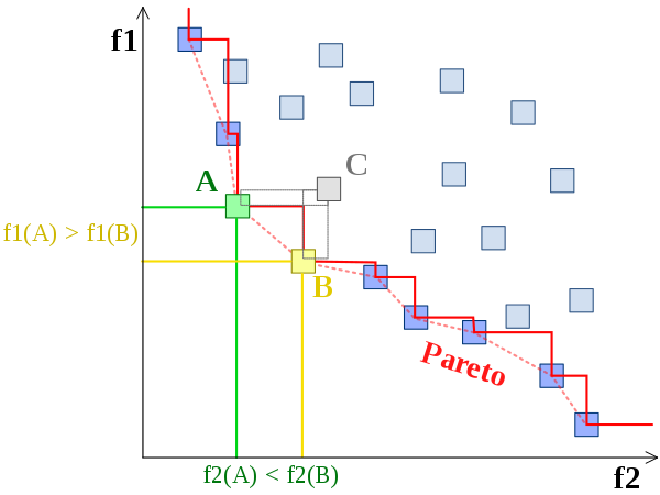
当解$ x_1 $和$ x_2 $满足以下两个条件时
* 对于所有的目标函数,$ f_i(x_1)\leq f_i(x_2) $,其中$ 1\leq i \leq k $
* 至少由一个目标函数$ f_i(x) $满足$ f_i(x_1) < f_i(x_2) $,其中$ 1\leq i \leq k $
我们称$ x_1 $支配$ x_2 $,如上图中$ A $和$ B $都支配$ C $,但彼此之间不存在支配关系。

当一个解集中任何一个解都不能被该集合中其他解支配,那么就称该解集为不可支配解集。一组帕累托最优结果,如上图中红色的边界,称为帕累托前沿或帕累托边界。

求解多目标优化问题的方法主要分为两类,一种是将多目标优化问题转换成单目标优化问题,常用的方法是对目标函数值加权求和或保留一个目标函数、其余的目标函数被转化为限定条件。但是由于实际应用中目标函数的函数值范围不好确定,因此转换成单目标优化算法的效果常常不好。实际应用更加广泛的是另一种采用多目标的优化算法。

多目标粒子群算法MOPSO

多目标粒子群算法最早由Coello等人提出[1],算法的大致处理步骤如下所示:
MOPSO

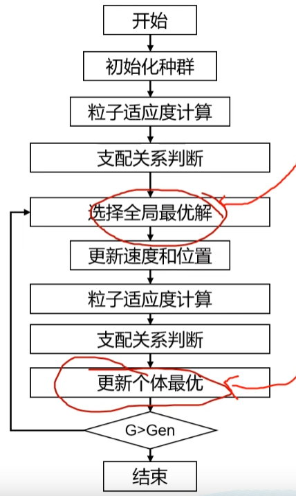
和粒子群算法不同的是,这里添加了支配关系判断的步骤,同时选择全局最优解以及更新个体最优的步骤和粒子群算法也有所不同。此外,MOPSO还额外维护了精英解和解空间的网格,下面我们将分别加以介绍。

首先是支配关系的判断,根据第一部分中对于帕累托前沿和支配关系的介绍,我们知道多目标优化问题中解的优劣由支配关系来加以判断。

每次迭代开始时,我们需要从精英解集合中选择当前的全局最优解,精英解中包含的是不被其他解支配的解的集合,换言之,精英解包含的是目前获取到的帕累托前沿。选择全局最优解的步骤如下:
1. 在解集空间中绘制网格,即根据当前的解集中不同目标函数的最大值和最小值,将空间均匀等分并给每个子空间添加索引,确定不同的解所对应的子空间。
2. 对于包含解的子空间,判断每个子空间中存在的解个数$ N_1,\cdots,N_k $,使用轮盘赌算法获取当前的全局最优解,轮盘赌的概率和解的个数呈反相关关系(让解稀疏的子空间拥有更大的被选中的概率,设法让解在帕累托前沿上分布更均匀)。

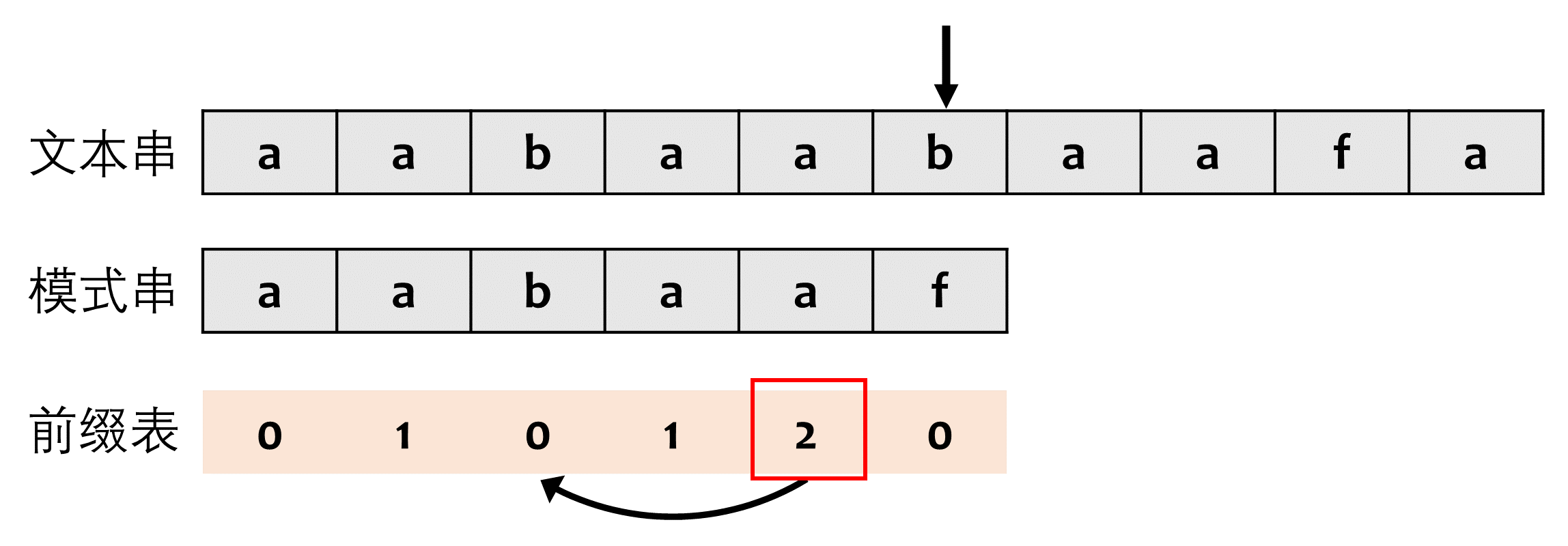
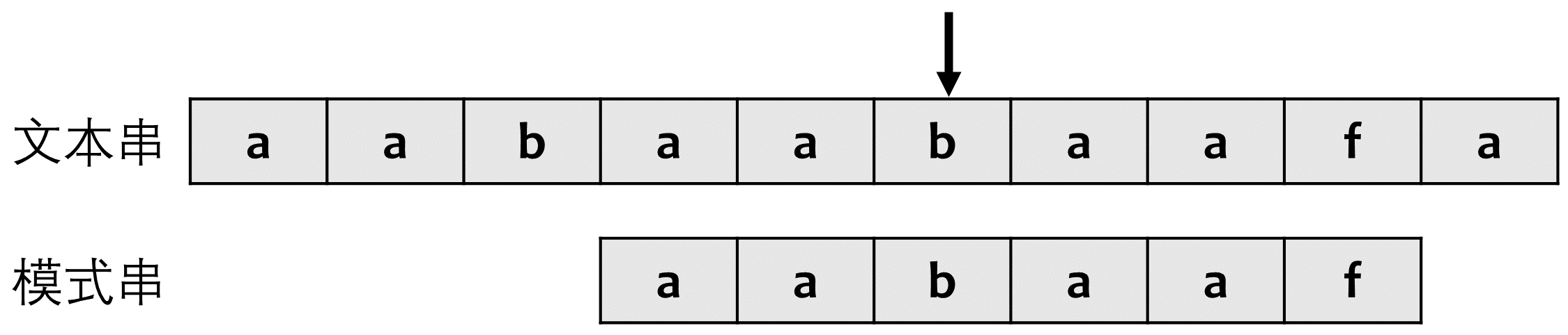
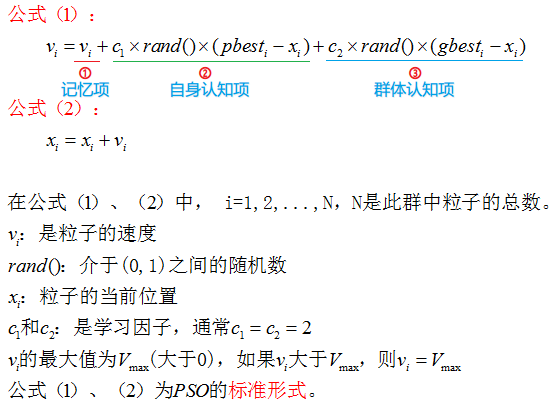
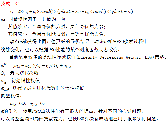
选择好当前的全局最优解后更新粒子的位置和速度,更新公式和粒子群算法一致。

$$v_i = w \times v_i + c_1\times rand() \times ((p_{best})_i-x_i) + c_2\times rand()\times ((g_{best})_i-x_i)$$

粒子更新后会根据粒子当前解和局部最优解之间的支配关系更新粒子的局部最优解。在更新局部最优解之前,还可以采取类似于遗传算法的步骤,以一定的概率对粒子的当前解进行变异。

更新完局部最优解之后更新精英解集合,保留当前不被其他解支配的解,同时为了避免精英解过大,可以设置一个阈值来控制精英解集合中的解数目,多余的精英解被随机抛弃。

多目标遗传算法NSGA-II

多目标遗传算法NSGA-II由Deb等人提出[2],算法的大致处理步骤如下所示:
NSGA-II
相较于单目标进化算法添加了快速非支配排序和父代、子代合并操作增加种群多样性,此外从$ rank_i $ 中取出一部分个体有两种方式、一种是拥挤距离排序、另一种是随机选择。下面我们将分别加以介绍。

对于当前已有的父代解和子代集合,融合两个集合产生当前的解集合,首先执行非支配排序,非支配排序的大致步骤为,先找出解集中的非支配边沿,将这部分的解的$ rank $置为1;去掉这部分解,继续找出剩下的解集中的非支配边沿,将这部分的解的$ rank $置为2,重复上述步骤知道遍历完所有的解。实际实现中需要记录每个解支配的解,方便后续的$ rank $计算,具体可以参考后面的参考代码实现。

在当前解集合中选取下一轮迭代的父代解集合。需要注意的是对于固定大小的父代解集合,这里依次从$ rank=1 $的解开始加入,知道数量满足要求。最后可能需要从$ rank=i $的解集合中选取一部分,此时有两种方式,一种是随机选取,一种是根据拥挤度距离排序后选取。拥挤度距离计算的示意图如下,
拥挤度距离
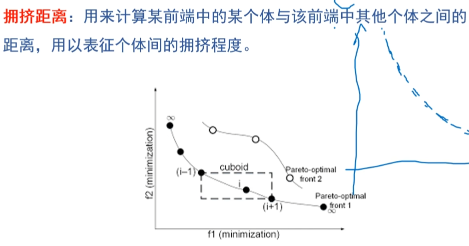
拥挤度距离可以用来衡量当前解周围的解的密度,优先选择拥挤度距离大(解稀疏)的地方可以使得最后求得的帕累托前沿上解分布更均匀。

对当前的解执行交叉变异操作产生下一轮迭代的子代解,交叉变异操作可以有不同的实现。

代码实现

目标函数

# -*- coding : utf-8 -*-
from collections import defaultdict
import math
import numpy as np

def ZDT1(x):
    """
    测试函数——ZDT1
    :parameter
    :param x: 为 m 维向量,表示个体的具体解向量
    :return f: 为两个目标方向上的函数值
    """
    poplength = len(x)
    f = defaultdict(float)

    g = 1 + 9 * sum(x[1:poplength]) / (poplength - 1)
    f[1] = x[0]
    f[2] = g * (1 - pow(x[0] / g, 0.5))

    return f

def ZDT2(x):
    poplength = len(x)
    f = defaultdict(float)

    g = 1 + 9 * sum(x[1:poplength]) / (poplength - 1)
    f[1] = x[0]
    f[2] = g * (1 - (x[0] / g) ** 2)

    return f


def KUR(x):
    f = defaultdict(float)
    poplength = len(x)

    f[1] = 0
    for i in range(poplength - 1):
        f[1] = f[1] + (-10) * math.exp((-0.2) * (x[i] ** 2 + x[i+1] ** 2) ** 0.5)

    for i in range(poplength):
        f[2] = abs(x[i]) ** 0.8 + 5 * math.sin(x[i] ** 3)

    return f


# 轮盘赌函数
def RouletteWheelSelection(P):
    idx = np.argsort(P)
    val = np.sort(P)
    prob = [_/sum(P) for _ in val]  # 概率
    dprob = np.cumsum(prob)  # 累积概率
    seed = np.random.random()  # 随机数

    res = idx[(dprob>seed).tolist().index(True)]  # 选择
    return res

MOPSO

参考了Matlab实现

# -*- coding: utf-8 -*-
# Lishengxie
# 2023-03-03
# Implementation of multi-objective particle swarm algorithm

from collections import defaultdict
import numpy as np
from utils import ZDT1, ZDT2, KUR, RouletteWheelSelection
import matplotlib.pyplot as plt
import copy

class Particle:
    """
    Implementation of particle class, which provides the constraints for particle's position and the method to compute dominance.
    """
    def __init__(self):
        self.position = None
        self.velocity = None
        self.best = None
        self.cost = defaultdict()
        self.is_dominated = False

    def bound_position(self, var_min, var_max):
        """
        对解向量 solution 中的每个分量进行定义域判断,超过最大值,将其赋值为最大值;小于最小值,赋值为最小值
        Args:
            var_min: 位置域下限
            var_max: 位置域上限
        Returns:
            None
        """
        self.position = np.clip(self.position, var_min, var_max)

    def update_position(self, var_min, var_max):
        """
        Update particle'sposition
        Args:
            var_min: 位置域下限
            var_max: 位置域上限
        Returns:
            None
        """
        self.position += self.velocity
        self.bound_position(var_min, var_max)

    def cal_cost(self, objective_func):
        """
        Calculate the objective scores.
        Args:
            objective_func: Function, return objective scores with position given.
        Return:
            cost: collection.defaultdict, cost function scores with keys from `1` to `N`.
        """
        return objective_func(self.position)

    def dominate(self, other):
        """
        Return the dominance relationship between the current particle and input particle. `A` dominates `B` if any of `A`'s cost is less than or equal to `B` and at least one of `A`'s cost is less than `B`.
        Args:
            other: Particle, the other particle to be compared
        """
        v1 = np.array(list(self.cost.values()))
        v2 = np.array(list(other.cost.values()))
        return (v1<=v2).all() and (v1<v2).any()

class MOPSO:
    """
    Multi-objective particle swarm optimization algorithm.
    """
    def __init__(self, max_iter=200, n_pop=200, n_rep=100,\
                 w=0.5, wdamp=0.99, c1=1., c2=2., n_grid=7, alpha=0.1,\
                 beta=2., gamma=2., mu=0.1, n_var=5, var_min=0., var_max=1., \
                 objective_func=ZDT1, objective_num=2):
        """
        Args:
            max_iter:       int, Maximum Number of Iterations
            n_pop:         int, Population Size
            n_rep:          int, Repository Size
            w:              float, Intertia Weight
            wdamp:          float, Intertia Weight Damping Rate
            c1:             float, Personal Learning Coefficient
            c2:             float, Global Learning Coefficient
            n_grid:         int, number of Grids per Dimension
            alpha:          float, Inflation Rate
            beta:           float, Leader Selection Pressure
            gamma:          float, Deletion Selection Pressure
            mu:             float, Mutation Rate
            n_var:          int, Number of decision variables
            var_max:        float, Lower Bound of Variables
            var_min:        float, Upper Bound of Variables
            objective_func: function, cost function to minimize
            objective_num:  int, number of cost function
        Returns:
            None
        """
        self.max_iter = max_iter
        self.n_pop = n_pop
        self.n_rep = n_rep
        self.w = w
        self.wdamp = wdamp
        self.c1 = c1
        self.c2 = c2
        self.n_grid = n_grid
        self.alpha = alpha
        self.beta = beta
        self.gamma = gamma
        self.mu = mu
        self.n_var = n_var
        self.var_max = var_max
        self.var_min = var_min
        self.objective_func = objective_func
        self.objective_num = objective_num

        # particle swam
        self.particles = []
        # repository, which stores the dominant particles on the Pareto Front
        self.repository = []
        # init particle swam
        self.init_particle()

        # grid matrix, avoiding the computation of crowding distance
        self.grid = np.zeros((self.objective_num, self.n_grid + 2))
        self.grid_index = None
        self.grid_subindex = None

    def init_particle(self):
        """
        Init particles with the number of `n_pop`
        """
        for i in range(self.n_pop):
            # init a particle
            p = Particle()
            p.position = np.random.random(self.n_var) * (self.var_max-self.var_min) + self.var_min
            p.velocity = np.zeros(self.n_var)
            # cost dict
            p.cost = p.cal_cost(self.objective_func)
            # local best solution
            p.best = Particle()
            p.best.position = p.position
            p.best.cost = p.cost
            # add particle to the particle swam
            self.particles.append(p)

    def determine_domination(self, pop):
        """
        Determine the dominance relationship in a given group of particles.
        Args:
            pop: List[Particle], group of particles
        """
        n_pop = len(pop)

        # reset all the `is_dominated` be False
        for i in range(n_pop):
            pop[i].is_dominated = False

        # traverse all of the particle pairs
        for i in range(n_pop-1):
            for j in range(i+1, n_pop):
                if pop[i].dominate(pop[j]):
                    pop[j].is_dominated = True
                if pop[j].dominate(pop[i]):
                    pop[i].is_dominated = True
        return pop

    def determine_repository(self, pop):
        """
        Add the particle `p` in `pop` to `repository` if `p` is not been dominated.
        Args:
            pop: List[Particle], group of particles 
        """
        for i in range(len(pop)):
            if not pop[i].is_dominated:
                self.repository.append(copy.deepcopy(pop[i]))

    def create_grid(self, pop):
        """
        Create grids in cost function space(2D or more), limited by the maximum and minimum value of cost funciton.
        Args:
            pop: List[Particle], group of particles
        """
        n_pop = len(pop)
        cost = np.zeros((self.objective_num, n_pop))
        # Get cost of each particle
        for c in range(1, self.objective_num+1):
            for i in range(n_pop):
                cost[c-1][i] = pop[i].cost[c]
        cmin = np.min(cost, axis=1)
        cmax = np.max(cost, axis=1)
        dc = cmax-cmin
        cmin = cmin - self.alpha * dc;
        cmax = cmax + self.alpha * dc;

        for j in range(self.objective_num):
            self.grid[j] = np.append(np.linspace(cmin[j], cmax[j], self.n_grid+1), np.inf)
        return cost

    def find_grid_index(self, pop, cost):
        """
        Find the grid index for each particle in the grids matrix, the multi-dimensional index is transfered to integer.
        Args:
            pop: List[Particle], group of particles
            cost: numpy.ndarray, cost function matrix for particles in `pop`.
        """
        n_pop = len(pop)
        self.grid_subindex = np.zeros((n_pop, self.objective_num), dtype=np.uint)
        self.grid_index = np.zeros((n_pop), dtype=np.uint)
        for i in range(n_pop):
            for j in range(self.objective_num):
                self.grid_subindex[i][j] = np.argwhere(self.grid[j] > cost[j][i])[0]
                if j == 0:
                    self.grid_index[i] = self.grid_subindex[i][j]
                else:
                    self.grid_index[i] = (self.grid_index[i]-1)*self.n_grid + self.grid_subindex[i][j]

    def select_leader(self):
        """
        Select a leader from `repository` based on the Roulette algorithm. More about the Roulette algorithm, refer to `https://blog.csdn.net/doubi1/article/details/115923275`
        """
        # occupied cells
        oc = np.unique(self.grid_index)
        # number of particles in the occupied cells
        N = np.zeros_like(oc)
        for i in range(len(N)):
            N[i] = np.sum(self.grid_index==oc[i])

        P = np.exp(-self.beta*N)
        P = P/np.sum(P)
        sel = RouletteWheelSelection(P)

        # selected cell
        sc = oc[sel]
        # selected cell members
        scm =  np.argwhere(self.grid_index==sc).flatten()
        # selected member
        sm = scm[np.random.randint(0, len(scm))]
        return self.repository[sm]

    def mutate(self, position, pm):
        """
        Select a particle `j`(randomly selected) to conduct mutation.
        Args:
            pm: float, mutation scale.
        """
        j = np.random.randint(0, self.n_var)
        dx = pm * (self.var_max - self.var_min)
        lb = position[j] - dx
        if lb < self.var_min:
            lb = self.var_min
        ub = position[j] + dx
        if ub > self.var_max:
            ub = self.var_max
        x_new = position
        x_new[j] = np.random.random() * (ub-lb) + lb
        return x_new

    def delete_one_rep_member(self):
        """
        Select a particle from `repository` and delete it.
        """
        # occupied cells
        oc = np.unique(self.grid_index)
        # number of particles in the occupied cells
        N = np.zeros_like(oc)
        for i in range(len(N)):
            N[i] = np.sum(self.grid_index==oc[i])

        P = np.exp(self.gamma*N)
        P = P/np.sum(P)
        sel = RouletteWheelSelection(P)
        # selected cell
        sc = oc[sel]
        # selected cell members
        scm =  np.argwhere(self.grid_index==sc).flatten()
        # selected member
        sm = scm[np.random.randint(0, len(scm))]
        self.repository[sm] = None

    def plot(self):
        X = []
        Y = []
        X2 = []
        Y2 = []
        for ind in self.particles:
            X.append(ind.cost[1])
            Y.append(ind.cost[2])
        for ind in self.repository:
            X2.append(ind.cost[1])
            Y2.append(ind.cost[2])
        # plt.xlim(0, 1)
        # plt.ylim(0, 1)
        plt.xlabel('F1')
        plt.ylabel('F2')
        plt.scatter(X, Y)
        plt.scatter(X2, Y2)

    def solve(self):
        """
        Execute the optimization process.
        """
        # Init step
        self.particles = self.determine_domination(self.particles)
        self.determine_repository(self.particles)
        cost = self.create_grid(self.repository)
        self.find_grid_index(self.repository, cost)

        # Main loop
        for it in range(self.max_iter):
            for i in range(self.n_pop):
                # select the global best particle
                leader = self.select_leader()
                # update particle's velocity and position
                self.particles[i].velocity = self.w * self.particles[i].velocity \
                                            + self.c1 * np.random.random(self.n_var) * (self.particles[i].best.position - self.particles[i].position) \
                                            + self.c2 * np.random.random(self.n_var) * (leader.position - self.particles[i].position) 
                self.particles[i].update_position(self.var_min, self.var_max)
                self.particles[i].cost = self.particles[i].cal_cost(self.objective_func)

                # Apply Mutation
                pm = (1-(it-1) / (self.max_iter - 1)) ** (1./self.mu)
                if np.random.random() < pm:
                    new_sol = Particle()
                    new_sol.position = self.mutate(self.particles[i].position, pm)
                    new_sol.cost = new_sol.cal_cost(self.objective_func)
                    if new_sol.dominate(self.particles[i]):
                        self.particles[i].position = new_sol.position
                        self.particles[i].cost = new_sol.cost
                    elif self.particles[i].dominate(new_sol):
                        pass
                    else:
                        if np.random.random() < 0.5:
                            self.particles[i].position = new_sol.position
                            self.particles[i].cost = new_sol.cost

                # update locate best solution
                if self.particles[i].dominate(self.particles[i].best):
                    self.particles[i].best.position = self.particles[i].position
                    self.particles[i].best.cost = self.particles[i].cost
                elif self.particles[i].best.dominate(self.particles[i]):
                    pass
                else:
                    if np.random.random() < 0.5:
                        self.particles[i].best.position = self.particles[i].position
                        self.particles[i].best.cost = self.particles[i].cost

            # update `repository`
            # for each in self.particles:
                # self.repository.append(each)
            self.determine_repository(self.particles)
            self.repository = self.determine_domination(self.repository)
            tmp = []
            for each in self.repository:
                if not each.is_dominated:
                    tmp.append(each)
            self.repository = tmp

            # update cost grid based on `repository`
            cost = self.create_grid(self.repository)
            self.find_grid_index(self.repository, cost)

            # delete particles randomly from `repository` which is out of capacity
            if len(self.repository) > self.n_rep:
                for _ in range(len(self.repository) - self.n_rep):
                    self.delete_one_rep_member()

            # update grid index for the next loop
            grid_index = []
            repository = []
            for i in range(len(self.repository)):
                if self.repository[i] is None:
                    continue
                else:
                    grid_index.append(self.grid_index[i])
                    repository.append(self.repository[i])
            self.grid_index = grid_index
            self.repository = repository

            plt.clf()
            plt.title('current iteration:' + str(it + 1))
            self.plot()
            plt.pause(0.01)

            print("Iteration {}: number of rep members = {}".format(it, len(self.repository)))
            self.w = self.w * self.wdamp
        plt.show()


if __name__ == "__main__":
    # mopso = MOPSO(objective_func=KUR, var_max=5, var_min=-5, n_var=3, max_iter=400, n_pop=100)
    mopso = MOPSO(objective_func=ZDT1)
    mopso.solve()

NSGA-II

参考了开源实现

#  -*-  coding  =  utf-8  -*-
from collections import defaultdict
import numpy as np
import random
import matplotlib.pyplot as plt
import math
from utils import ZDT1, ZDT2, KUR


class Individual(object):
    def __init__(self):
        self.solution = None  # 实际赋值中是一个 nparray 类型,方便进行四则运算
        self.objective = defaultdict()

        self.n = 0          # 解p被几个解所支配,是一个数值(左下部分点的个数)
        self.rank = 0       # 解所在第几层
        self.S = []         # 解p支配哪些解,是一个解集合(右上部分点的内容)
        self.distance = 0   # 拥挤度距离

    def bound_process(self, bound_min, bound_max):
        """
        对解向量 solution 中的每个分量进行定义域判断,超过最大值,将其赋值为最大值;小于最小值,赋值为最小值
        :param bound_min: 定义域下限
        :param bound_max: 定义域上限
        :return:
        """
        for i, item in enumerate(self.solution):
            if item > bound_max:
                self.solution[i] = bound_max
            elif item < bound_min:
                self.solution[i] = bound_min

    def calculate_objective(self, objective_fun):
        self.objective = objective_fun(self.solution)

    # 重载小于号“<”
    def __lt__(self, other):
        v1 = list(self.objective.values())
        v2 = list(other.objective.values())
        for i in range(len(v1)):
            if v1[i] > v2[i]:
                return 0  # 但凡有一个位置是 v1大于v2的 直接返回0,如果相等的话比较下一个目标值
        return 1

    # 重载大于号“>”
    def __gt__(self, other):
        v1 = list(self.objective.values())
        v2 = list(other.objective.values())
        for i in range(len(v1)):
            if v1[i] < v2[i]:
                return 0  # 但凡有一个位置是 v1小于v2的 直接返回0
        return 1


class NSGAII:
    def __init__(self, max_iter=200, n_pop=100, n_var=30,\
                  eta=1, var_min=0, var_max=1, objective_fun = ZDT1):
        """
        Args:
            max_iter:       int, Maximum Number of Iterations
            n_pop:          int, Population Size
            eta:            float, 变异分布参数,该值越大则产生的后代个体逼近父代的概率越大;Deb建议设为 1
            n_var:          int, Number of decision variables
            var_max:        float, Lower Bound of Variables
            var_min:        float, Upper Bound of Variables
            objective_func: function, cost function to minimize
        Returns:
            None
        """
        self.max_iter = max_iter
        self.n_pop = n_pop
        self.n_var = n_var
        self.eta = eta
        self.var_min = var_min
        self.var_max = var_max
        self.objective_fun = objective_fun

        self.P = []
        self.init_P()

    def init_P(self):
        for i in range(self.n_pop):
            self.P.append(Individual())
            # 随机生成个体可行解
            self.P[i].solution = np.random.rand(self.n_var) * (self.var_max - self.var_min) + self.var_min  
            self.P[i].bound_process(self.var_min, self.var_max)  # 定义域越界处理
            self.P[i].calculate_objective(self.objective_fun)  # 计算目标函数值

    def fast_non_dominated_sort(self, P):
        """
        非支配排序
        :param P: 种群 P
        :return F: F=(F_1, F_2, ...) 将种群 P 分为了不同的层, 返回值类型是dict,键为层号,值为 List 类型,存放着该层的个体
        """
        F = defaultdict(list)

        for p in P:
            p.S = []
            p.n = 0
            for q in P:
                if p < q:  # if p dominate q
                    p.S.append(q)  # Add q to the set of solutions dominated by p
                elif q < p:
                    p.n += 1  # Increment the domination counter of p
            if p.n == 0:
                p.rank = 1
                F[1].append(p)

        i = 1
        while F[i]:
            Q = []
            for p in F[i]:
                for q in p.S:
                    q.n = q.n - 1
                    if q.n == 0:
                        q.rank = i + 1
                        Q.append(q)
            i = i + 1
            F[i] = Q

        return F

    def crowding_distance_assignment(self, L):
        """ 传进来的参数应该是L = F(i), 类型是List"""
        l = len(L)  # number of solution in 
        for i in range(l):
            L[i].distance = 0  # initialize distance

        for m in L[0].objective.keys():
            L.sort(key=lambda x: x.objective[m])  # sort using each objective value
            L[0].distance = float('inf')
            L[l - 1].distance = float('inf')  # so that boundary points are always selected

            # 排序是由小到大的,所以最大值和最小值分别是 L[l-1] 和 L[0]
            f_max = L[l - 1].objective[m]
            f_min = L[0].objective[m]

            for i in range(1, l - 1):  # for all other points
                L[i].distance = L[i].distance + (L[i + 1].objective[m] - L[i - 1].objective[m]) / (f_max - f_min)

            # 虽然发生概率较小,但为了防止除0错,当bug发生时请替换为以下代码
            # if f_max != f_min:
            #     for i in range(1, l - 1):  # for all other points
            #         L[i].distance = L[i].distance + (L[i + 1].objective[m] - L[i - 1].objective[m]) / (f_max - f_min)

    def binary_tournament(self, ind1, ind2):
        """
        二元锦标赛
        :param ind1:个体1号
        :param ind2: 个体2号
        :return:返回较优的个体
        """
        if ind1.rank != ind2.rank:  # 如果两个个体有支配关系,即在两个不同的rank中,选择rank小的
            return ind1 if ind1.rank < ind2.rank else ind2
        elif ind1.distance != ind2.distance:  # 如果两个个体rank相同,比较拥挤度距离,选择拥挤读距离大的
            return ind1 if ind1.distance > ind2.distance else ind2
        else:  # 如果rank和拥挤度都相同,返回任意一个都可以
            return ind1

    def make_new_pop(self, P, eta, bound_min, bound_max, objective_fun):
        """
        use select,crossover and mutation to create a new population Q
        :param P: 父代种群
        :param eta: 变异分布参数,该值越大则产生的后代个体逼近父代的概率越大。Deb建议设为 1
        :param bound_min: 定义域下限
        :param bound_max: 定义域上限
        :param objective_fun: 目标函数
        :return Q : 子代种群
        """
        popnum = len(P)
        Q = []
        # binary tournament selection
        for i in range(int(popnum / 2)):
            # 从种群中随机选择两个个体,进行二元锦标赛,选择出一个 parent1
            i = random.randint(0, popnum - 1)
            j = random.randint(0, popnum - 1)
            parent1 = self.binary_tournament(P[i], P[j])

            # 从种群中随机选择两个个体,进行二元锦标赛,选择出一个 parent2
            i = random.randint(0, popnum - 1)
            j = random.randint(0, popnum - 1)
            parent2 = self.binary_tournament(P[i], P[j])

            while (parent1.solution == parent2.solution).all():  # 如果选择到的两个父代完全一样,则重选另一个
                i = random.randint(0, popnum - 1)
                j = random.randint(0, popnum - 1)
                parent2 = self.binary_tournament(P[i], P[j])

            # parent1 和 parent1 进行交叉,变异 产生 2 个子代
            Two_offspring = self.crossover_mutation(parent1, parent2, eta, bound_min, bound_max, objective_fun)

            # 产生的子代进入子代种群
            Q.append(Two_offspring[0])
            Q.append(Two_offspring[1])
        return Q


    def crossover_mutation(self, parent1, parent2, eta, bound_min, bound_max, objective_fun):
        """
        交叉方式使用二进制交叉算子(SBX), 变异方式采用多项式变异(PM)
        :param parent1: 父代1
        :param parent2: 父代2
        :param eta: 变异分布参数, 该值越大则产生的后代个体逼近父代的概率越大。Deb建议设为 1
        :param bound_min: 定义域下限
        :param bound_max: 定义域上限
        :param objective_fun: 目标函数
        :return: 2 个子代
        """
        poplength = len(parent1.solution)

        offspring1 = Individual()
        offspring2 = Individual()
        offspring1.solution = np.empty(poplength)
        offspring2.solution = np.empty(poplength)

        # 二进制交叉
        for i in range(poplength):
            rand = random.random()
            beta = (rand * 2) ** (1 / (eta + 1)) if rand < 0.5 else (1 / (2 * (1 - rand))) ** (1.0 / (eta + 1))
            offspring1.solution[i] = 0.5 * ((1 + beta) * parent1.solution[i] + (1 - beta) * parent2.solution[i])
            offspring2.solution[i] = 0.5 * ((1 - beta) * parent1.solution[i] + (1 + beta) * parent2.solution[i])

        # 多项式变异
        # TODO 变异的时候只变异一个,不要两个都变,不然要么出现早熟现象,要么收敛速度巨慢 why?
        for i in range(poplength):
            mu = random.random()
            delta = 2 * mu ** (1 / (eta + 1)) if mu < 0.5 else (1 - (2 * (1 - mu)) ** (1 / (eta + 1)))
            offspring1.solution[i] = offspring1.solution[i] + delta

        # 定义域越界处理
        offspring1.bound_process(bound_min, bound_max)
        offspring2.bound_process(bound_min, bound_max)

        # 计算目标函数值
        offspring1.calculate_objective(objective_fun)
        offspring2.calculate_objective(objective_fun)

        return [offspring1, offspring2]

    def solve(self):
        # 否 -> 非支配排序
        self.fast_non_dominated_sort(self.P)
        Q = self.make_new_pop(self.P, self.eta, self.var_min, self.var_max, self.objective_fun)

        P_t = self.P  # 当前这一届的父代种群
        Q_t = Q  # 当前这一届的子代种群

        for gen_cur in range(self.max_iter):
            R_t = P_t + Q_t  # combine parent and offspring population
            F = self.fast_non_dominated_sort(R_t)

            P_n = []  # 即为P_t+1,表示下一届的父代
            i = 1
            while len(P_n) + len(F[i]) < self.n_pop:  # until the parent population is filled
                self.crowding_distance_assignment(F[i])  # calculate crowding-distance in F_i
                P_n = P_n + F[i]  # include ith non dominated front in the parent pop
                i = i + 1  # check the next front for inclusion
            F[i].sort(key=lambda x: x.distance)  # sort in descending order using <n,因为本身就在同一层,所以相当于直接比拥挤距离
            P_n = P_n + F[i][:self.n_pop - len(P_n)]
            Q_n = self.make_new_pop(P_n, self.eta, self.var_min, self.var_max,
                            self.objective_fun)  # use selection,crossover and mutation to create a new population Q_n

            # 求得下一届的父代和子代成为当前届的父代和子代,,进入下一次迭代 《=》 t = t + 1
            P_t = P_n
            Q_t = Q_n

            # 绘图
            plt.clf()
            plt.title('current generation:' + str(gen_cur + 1))
            self.plot_P(P_t)
            plt.pause(0.1)

        plt.show()

        return 0

    def plot_P(self, P):
        """
        假设目标就俩,给个种群绘图
        :param P:
        :return:
        """
        X = []
        Y = []
        X1 = []
        Y1 = []
        for ind in P:
            X.append(ind.objective[1])
            Y.append(ind.objective[2])
            if ind.rank == 1:
                X1.append(ind.objective[1])
                Y1.append(ind.objective[2])

        plt.xlabel('F1')
        plt.ylabel('F2')
        plt.scatter(X, Y)
        plt.scatter(X1, Y1)


    def show_some_ind(self, P):
        # 测试使用
        for i in P:
            print(i.solution)


if __name__ == '__main__':
    solver = NSGAII()
    solver.solve()

参考文献

[1] Coello C A C, Lechuga M S. MOPSO: A proposal for multiple objective particle swarm optimization[C]//Proceedings of the 2002 Congress on Evolutionary Computation. CEC'02 (Cat. No. 02TH8600). IEEE, 2002, 2: 1051-1056.
[2] Deb K, Pratap A, Agarwal S, et al. A fast and elitist multiobjective genetic algorithm: NSGA-II[J]. IEEE transactions on evolutionary computation, 2002, 6(2): 182-197.

]]>
<![CDATA[启发式优化算法学习-模拟退火]]> https://www.lishengxie.top/index.php/archives/72/ 2023-02-27T11:06:00+08:00 2023-02-27T11:06:00+08:00 lishengxie https://www.lishengxie.top/

模拟退火算法(SA)

参考教程 https://blog.csdn.net/brilliantZC/article/details/124436967

模拟退火算法(Simulated Annealing,SA)是一种模拟物理退火过程而设计的优化算法。模拟退火算法采用类似于物理退火的过程。先在一个高温状态下(算法初始化随机解),然后逐渐退火,在每个温度下慢慢冷却,最终达到物理基态(相当于算法找到最优解)。模拟退火算法采用Metropolis准则,并用一组称为冷却进度表的参数控制算法的进程,使得算法在多项式时间里可以给出一个近似最优解。

SA算法运行流程

step1: 设定当前解(即为当前的最优解):令$ T =T_0 $,即开始退火的初始温度,随机生成一个初始解$ x_0 $,并计算相应的目标函数值$ E(x_0) $。
step2: 产生新解与当前解差值:根据当前解$ x_i $进行扰动,产生一个新解$ x_j $,计算相应的目标函数值$ E(x_j)$,得到$ \Delta E = E(x_j)-E(x_i)$。
step3: 判断新解是否被接受 :若$ \Delta E \leq 0 $,则新解$ x_j $被接受;若$ \Delta E> 0 $,则新解$ x_j $按概率$ e^{\frac{-(E(x_j)-E(x_i))}{T_i}} $被接受,$ T_i $为当前温度。
step4: 当新解被确定接受时,新解$ x_j $被作为当前解。
step5: 循环以上四个步骤:在温度$ T_i $下,重复$ k $次的扰动和接受过程,接着执行下一步骤。
step6: 最后找到全局最优解:判断$ T $是否已经达到终止温度$ T_f $,是,则终止算法;否,则转到循环步骤继续执行。

SA算法求解映射问题

映射问题本质上可以看作一个序列的排序问题,使用SA算法求解时,需要关注的是如何产生新解,这里我们采用如下的方法:再序列中随机选取两个不重合的位置,将这两个位置中间的序列反转达到局部扰动的目的。

SA算法求解映射问题代码

# -*- coding: utf-8 -*-
# Lishengxie
# 2023-02-23
# Implementation of a Simulated Annealing algorithm for crossbar mapping/placing
# 参考链接: https://blog.csdn.net/weixin_58427214/article/details/125901431
# 参考链接: https://blog.csdn.net/brilliantZC/article/details/124436967

import numpy as np
import copy
import sys
import random

class SAPlacer:
    """
        SA algorithm
        -------------
        Class used to find the mapping from computing cores to routers on NoC which minizes the communication cost
    """
    def __init__(self, dim_x, dim_y, spike_table, L=200, K=0.95, S=0.04, T=100, T_threshold=0.01):
        """
            Initialization of PsoPlacer.
            Args:
                dim_x: int, the `x` dimension on NoC 
                dim_y: int, the `y` dimension on NoC 
                spike_table: 2D-array, the number of spikes between core `i` and core `j`
                L: int, 每个温度下的迭代次数
                K: float, 温度的衰减参数, T = K*T
                S: float, 步长因子
                T: float, 初始温度
                T_threshold: float, 终止温度
        """
        self.dim_x = dim_x
        self.dim_y = dim_y
        self.dim_size = dim_x * dim_y
        self.L = L
        self.K = K
        self.S = S
        self.T = T
        self.T_threshold = T_threshold
        if spike_table is not None:
            self.init_solution(spike_table)

    def init_solution(self, spike_table):
        """
            Init spike table, hop distance table and solution.
        """
        # init spike table
        self.spike_table = np.zeros((self.dim_size, self.dim_size))
        h, w = spike_table.shape
        for i in range(h):
            for j in range(w):
                self.spike_table[i,j] = spike_table[i,j]

        # init hop distance table
        self.hop_xy()

        # init solution
        self.pre_x = np.arange(self.dim_size)
        np.random.shuffle(self.pre_x)
        self.pre_bestx = self.pre_x
        self.pre_x = np.arange(self.dim_size)
        np.random.shuffle(self.pre_x)
        self.prex_cost = self.fitnessFuntcion(self.pre_x)
        self.bestx = self.pre_x
        self.bestx_cost = self.fitnessFuntcion(self.bestx)

    def hop_xy(self):
        """
            The hop distance between router `x` and `y` in the 2D-Mesh NoC using XY routing
        """
        self.hop_dist = np.zeros((self.dim_size, self.dim_size))
        for i in range(self.dim_size):
            for j in range(self.dim_size):
                self.hop_dist[i,j] = abs(i % self.dim_x - j % self.dim_x) \
                                + abs(i // self.dim_x - j // self.dim_x)

    def fitnessFuntcion(self, solution):
        """
            Compute the communication cost for each mapping solution
            Args:
                solution: List, a possible mapping solution
        """
        cost = 0
        for i in range(self.dim_size):
            for j in range(self.dim_size):
                cost +=  self.spike_table[i,j] * self.hop_dist[solution[i], solution[j]]
        return cost

    def place(self):
        """
            Execute the Simulated Annealing algorithm
        """
        P = 0
        next_x = np.arange(self.dim_size)
        np.random.shuffle(next_x)
        nextx_cost = self.fitnessFuntcion(next_x)

        while (self.T > self.T_threshold):
            self.T = self.K * self.T        # 降温
            # 当前温度T下迭代次数
            for i in range(self.L):
                # ====在此点附近随机选下一点=====
                # 选择两个随机位置, 将两个位置之间的数组进行翻转
                positions = np.random.choice(list(range(self.dim_size)), replace=False, size=2)
                x = min(positions[0], positions[1])
                y = max(positions[0], positions[1])
                mid_reversed = next_x[x:y+1][::-1]
                next_x[x:y+1] = mid_reversed

                if random.random() <= 0.0001:
                    np.random.shuffle(next_x)

                nextx_cost = self.fitnessFuntcion(next_x)
                if nextx_cost < self.bestx_cost:
                    self.pre_bestx = self.bestx
                    self.bestx = next_x
                    self.bestx_cost = nextx_cost

                if nextx_cost < self.prex_cost:
                    self.pre_x = next_x
                    self.prex_cost = nextx_cost
                    P = P + 1
                else:
                    changer = -1 * (nextx_cost - self.prex_cost) / self.T
                    p1 = np.exp(changer)
                    if p1 > np.random.random():
                        self.pre_x = next_x
                        self.prex_cost = nextx_cost
                        P = P + 1

            print("Current T: {:.7f}, best cost: {}".format(self.T, self.bestx_cost))

        return self.bestx
]]>
<![CDATA[启发式优化算法学习-PSO]]> https://www.lishengxie.top/index.php/archives/69/ 2023-02-25T15:06:00+08:00 2023-02-25T15:06:00+08:00 lishengxie https://www.lishengxie.top/

粒子群算法(PSO)

参考教程:https://cloud.tencent.com/developer/article/1424756

粒子群算法是一种利用群体智能建立的一个简化模型,基于群体中个体对信息的共享使整个群体的运动趋向最优解。粒子群算法使用一群粒子,粒子拥有位置和速度两种属性,根据自身已经找到的最优解和参考整个共享于整个集群中找到的最优解去改变自己的飞行速度和位置。

粒子速度和位置

粒子群算法使用一定数量的粒子,粒子$ i $在$ N $维空间中的位置和速度表示为$ x_i=(x_1,x_2,\cdots,x_N) $ 和 $ v_i=(v_1,v_2,\cdots,v_N) $。每个粒子都有一个目标函数决定的适应值(fitness value),并且知道自己到目前为止发现的最好位置(pbest)和现在的位置$ x_i $。这个可以看作是粒子自己的飞行经验。除此之外,每个粒子还知道到目前为止整个群体中所有粒子发现的最好位置(gbest)(gbest是pbest中的最好值),这个可以看作是粒子同伴的经验。粒子就是通过自己的经验和同伴中最好的经验来决定下一步的运动。

粒子速度和位置更新公式

粒子群算法会给每个粒子一个初始的随机解,并通过迭代寻找最优解,迭代规则如下图所示:
PSO更新规则
迭代公式中的第一部分和第二部分分别反映了粒子对自身经验和群体经验的学习。基于上述公式还可以对当前的速度引入更新权重
PSO权重迭代

PSO算法运行流程

1)初始化一群微粒(群体规模为N),包括随机位置和速度;
2)评价每个微粒的适应度;
3)对每个微粒,将其适应值与其经过的最好位置pbest作比较,如果较好,则将其作为当前的最好位置pbest;
4)对每个微粒,将其适应值与其经过的最好位置gbest作比较,如果较好,则将其作为当前的最好位置gbest;
5)根据公式(2)、(3)调整微粒速度和位置;
6)未达到结束条件则转第2)步。
迭代终止条件根据具体问题一般选为最大迭代次数Gk或(和)微粒群迄今为止搜索到的最优位置满足预定最小适应阈值。

PSO算法求解映射问题

映射问题本质上可以看作一个序列的排序问题,使用PSO算法求解映射问题时,粒子位置对应一个序列的排序。这里$ pbest-x_i^{t-1} $对应将$ x_i^{t-1} $转换成pbest所需要的交换序列,这里的迭代公式的含义变为对于原来的解序列$ x_i^{t-1} $,

  • 先按照$ c_2 $的概率使用$ pbest-x_i^{t-1} $的交换序列对$ x_i^{t-1} $进行交换获得$ (x_i^{t-1})^{'} $,
  • 再按照$ c_3 $的概率使用$ gbest-(x_i^{t-1})^{'} $的交换序列对$ (x_i^{t-1})^{'} $进行交换获得$ x_i^{t} $.

PSO求解映射代码

# -*- coding: utf-8 -*-
# Lishengxie
# 2023-02-19
# Implementation of a PSO algorithm for crossbar mapping/placing

import numpy as np
import copy
import sys

class PsoPlacer:
    """
        PSO algorithm
        -------------
        Class used to find the mapping from computing cores to routers on NoC which minizes the communication cost
    """
    def __init__(self, dim_x, dim_y, spike_table, num_particle=50, s1=1.0, s2=0.04, s3=0.02):
        """
            Initialization of PsoPlacer.
            Args:
                dim_x: int, the `x` dimension on NoC 
                dim_y: int, the `y` dimension on NoC 
                spike_table: 2D-array, the number of spikes between core `i` and core `j`
                num_particle: int, number of particles in the PSO algorithm
        """
        self.dim_x = dim_x
        self.dim_y = dim_y
        self.dim_size = dim_x * dim_y
        self.num_particle = num_particle
        self.s1 = s1
        self.s2 = s2
        self.s3 = s3
        self.init_particle(spike_table)

    def init_particle(self, spike_table):
        """
            Init spike table, particles, local and global best solution
            Args:
                spike_table: 2D-array, the number of spikes between core `i` and core `j`
        """
        # init the spike table, adding `0`s if the dimension of `spike_table` not equal to `dim_size`
        self.spike_table = np.zeros((self.dim_size, self.dim_size))
        h, w = spike_table.shape
        for i in range(h):
            for j in range(w):
                self.spike_table[i,j] = spike_table[i,j]

        # init particle vectors with number of `num_particle`, each vector is a mappinng solution
        self.solution = np.zeros((self.num_particle, self.dim_size), dtype=np.int32)
        for i in range(self.num_particle):
            self.solution[i] = np.arange(self.dim_size)
            np.random.shuffle(self.solution[i])

        # init hop distance table
        self.hop_xy()

        # init the local/global best solution and their cost
        self.local_best_solution = copy.deepcopy(self.solution)
        self.local_best_cost = np.zeros((self.num_particle,))
        self.global_best_solution = np.arange(self.dim_size)
        self.global_best_cost = sys.maxsize
        for i in range(self.num_particle):
            self.local_best_cost[i] = self.fitnessFuntcion(self.local_best_solution[i])
            if self.local_best_cost[i] < self.global_best_cost:
                self.global_best_solution = self.local_best_solution[i]
                self.global_best_cost = self.local_best_cost[i]
        print("Init, gloabal best cost:{}".format(self.global_best_cost))


    def hop_xy(self):
        """
            The hop distance between router `x` and `y` in the 2D-Mesh NoC using XY routing
        """
        self.hop_dist = np.zeros((self.dim_size, self.dim_size))
        for i in range(self.dim_size):
            for j in range(self.dim_size):
                self.hop_dist[i,j] = abs(i % self.dim_x - j % self.dim_x) \
                                + abs(i // self.dim_x - j // self.dim_x)

    def fitnessFuntcion(self, solution):
        """
            Compute the communication cost for each mapping solution
            Args:
                solution: List, a possible mapping solution
        """
        cost = 0
        for i in range(self.dim_size):
            for j in range(self.dim_size):
                cost +=  self.spike_table[i,j] * self.hop_dist[solution[i], solution[j]]
        return cost

    def compute_swap_sequence(self, src_seq, dst_seq, seq_len):
        # TODO: Optimize this algorithm.
        """
            Find the swap sequence from source sequecne to destination sequence.
            Args:
                src_seq: List, the source sequence
                dst_seq: List, the destination sequence
                seq_len: int, the length of source and destination sequence
            Return:
                swap_sequence: the index of each point for `src_seq` in `dst_seq`
        """
        swap_seq = np.zeros((seq_len,))
        for i in range(seq_len):
            swap_seq[i] = np.where(dst_seq == src_seq[i])[0]
        return swap_seq

    def applySwap(self, swap_seq, src_seq, seq_len):
        """
            Apply swap sequence to the source sequence
            Args:
                src_seq: List, the source sequence
                swap_sequence: the index of each point for `src_seq` in `dst_seq`
                seq_len: int, the length of source and destination sequence
            Return:
                dst_seq: List, the destination sequence
        """
        dst_seq = np.zeros((seq_len,))
        for i in range(seq_len):
            dst_seq[swap_seq[i]] = src_seq[i]
        return dst_seq

    def place(self, num_iter=10):
        """
            Funciton to execute pso algorithm.
            Args:
                num_iter: int, max number of iterations to execute pso update
            Return:
                global best solution after `num_iter` iterations
        """
        for iter in range(num_iter):
            for i in range(self.num_particle):
                tmp_solution = copy.deepcopy(self.solution[i])
                if np.random.random() <= self.s2:
                    # print("local")
                    swap_seq_local = self.compute_swap_sequence(tmp_solution, self.local_best_solution[i], self.dim_size)
                    self.solution[i] = self.applySwap(self.solution[i], swap_seq_local, self.dim_size)
                if np.random.random() <= self.s3:
                    # print("global")
                    swap_seq_global = self.compute_swap_sequence(tmp_solution, self.global_best_solution, self.dim_size)
                    self.solution[i] = self.applySwap(self.solution[i], swap_seq_global, self.dim_size)

                if np.random.random() <= 0.0001:
                    np.random.shuffle(self.solution[i])

                cost = self.fitnessFuntcion(self.solution[i])
                if cost < self.local_best_cost[i]:
                    self.local_best_cost[i] = cost
                    self.local_best_solution[i] = copy.deepcopy(self.solution[i])

                if self.local_best_cost[i] < self.global_best_cost:
                    self.global_best_cost = self.local_best_cost[i]
                    self.global_best_solution = copy.deepcopy(self.local_best_solution[i])
            print("Iteration:{}, global best cost:{}".format(iter, self.global_best_cost))
        return self.global_best_solution
]]>